How to Use IMPORTHTML Function in Google Sheets?

When working with Google Sheets, we may want to import tables or lists from the pages we browse the internet on our own. No need to bother with copy-paste. Because format it again is a waste of time.
We can easily do this with IMPORTHTML. It is a very useful function, especially for use in data visualizations.
Let's have a study where we look at the relationship with the life expectancy of country X and GDP per capita or let's study the ratio of male and female populations in countries to the general population.
The syntax of the function is pretty easy. It is enough to know the URL of the page we are working with and what we want to receive. Let's explain the syntax and how the function works through an example.
What is the syntax for the IMPORTHTML function?
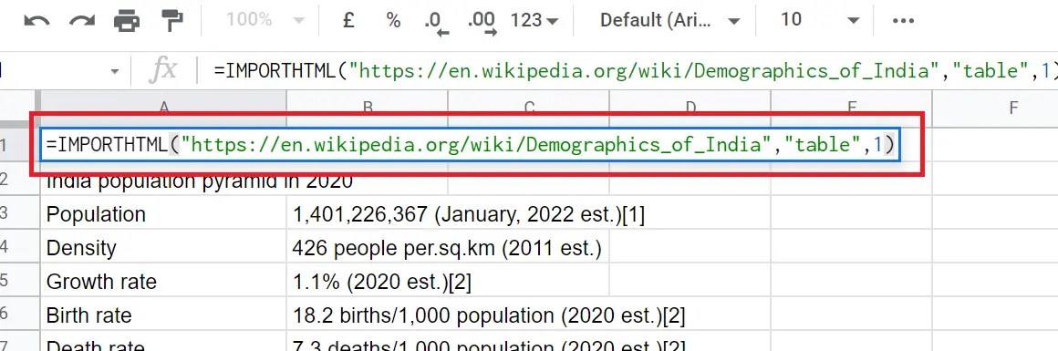
Let's explain the syntax through the screenshot above. We will bring the tables or lists on the Wikipedia page, which are offered as suggestions on our Google sheets worksheet, to our page.
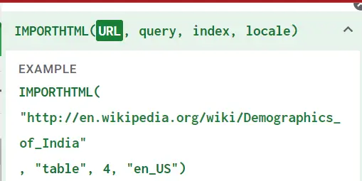
=IMPORTHTML(“URL”,”query”, index,locale)

=IMPORTHTML("https://en.wikipedia.org/wiki/Demographics_of_India","table",1)
- URL: ”https://en.wikipedia.org/wiki/Demographics_of_India“
- Query(Table or list): There are many tables and lists on the Wikipedia page. We will choose a table or list according to our request. I wanted a table in the example.
- Index: There may be more than one table on the page where we want to retrieve the data. In such a case, we must enter the order of the table we want. In the example, I entered it as '1' because I wanted the first table on the page.
- Locale: The language to be used when retrieving the data. If not specified, the local language is selected.
That's it for the function. Now let's take a look at the new version of our worksheet.
After the data come to our page, we cannot make any changes to it. If we want to make such a change,
Right click->Copy->Paste special-Values only


