How to Use VLOOKUP Function in Google Sheets?

When working with Google Sheets, we can have multiple tables, multiple sheets, or multiple workbooks. Among these, we may need to work with identical columns and corresponding columns.

For example, product codes, product names. We may need to use them on multiple pages. Instead of moving columns every time, we can easily handle this with VLOOKUP.

The table we have contains the names, product codes, and sales codes of the products sold. We will do the work in three parts, on the same page, in different numbers, and in different workbooks.

How to use the VLOOKUP function within the same worksheet?

There is a section that I have taken from the supermarket dataset I have. I want to see the product codes corresponding to the order numbers of the products.

We will use VLOOKUP for this. Let's write the function first. Then I will explain the places in the formula one by one. I will explain through the table below.

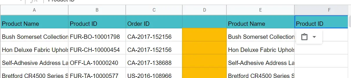
I want the product id corresponding to the product names. Come to cell F2 and write the following formula.

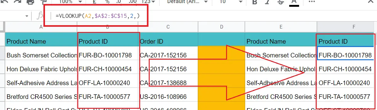
=VLOOKUP (A2, A2:C15,2,)

• A2 → Cell with the name corresponding to my product code.
• A2:C15 → The cell range to search for my product id. It will be healthier if we press F4. The result does not change even when the table is copied. $A$2:$C$15. Pressing F4 while selecting the range of cells we are typing prints like this.
• 2→I wrote the 2nd column because I want the product id.

Future result of columns:

• Column 1->Product name
• Column 2 ->Product ID
• Column 3->Order ID

After the column selection, we choose True or False. If we leave the ',' blank, it will be perceived as False. That is, it returns the exact equivalent. Writing False and leaving it blank have the same meaning.

How to use VLOOKUP to get data from another sheet?

We can also import data from another sheet in the same workbook. We will use =VLOOKUP for this. The syntax will still be the same. Let's take an example and explain it through an example.

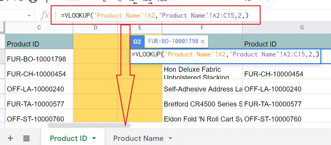
=VLOOKUP('Product Name'!A2,'Product Name'!A2:C15,2,)

1. =VLOOKUP( Go to the page where you want the information to come. I went to the 'Product Name' page.
2. 'Product Name'!A2→ The sheet name with the name corresponding to my product codes and the cell in that sheet.Select A2. Because your product names start from that cell. After selecting A2, the formula on the other page is filled automatically.
3. ''Product Name'!A2:C15' → The range of cells you want to search. My table is located between cells A2 and C15. If the above steps are followed exactly, the formula on the other page will be filled automatically.
4. 2, )→  Is the column where I want the information to come in. I wrote 2 because my product ids are in the 2nd column. I put ',' and left it blank so that the information corresponds exactly. This means the same as 'false' (,false= , )

• Column 1→ Product name
• Column 2 → Product ID
• Column 3→ Order ID

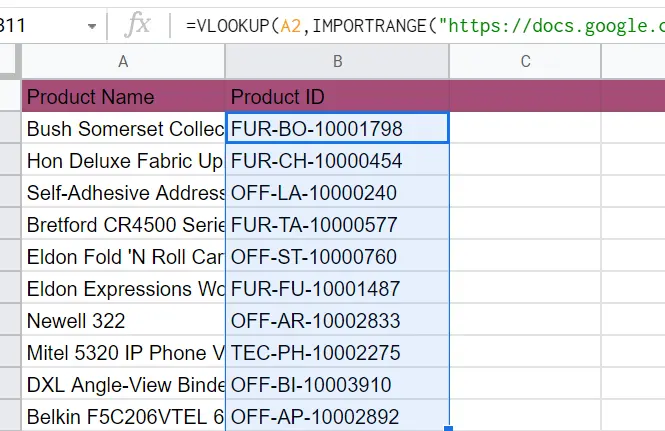
Here I have brought my product codes on the other page. I will add the table I use here and explain it with a video. You can practice and practice the same way.

How to use VLOOKUP to get data from another worksheet?

We have two workbooks. Here again, I will use the same worksheet. The syntax is a little different here. Let's do the example first. I will explain through example.

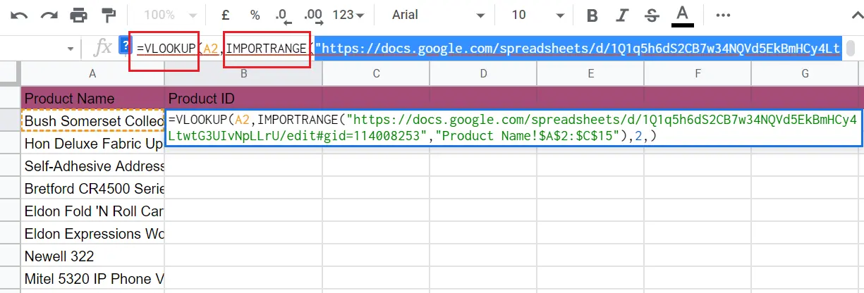
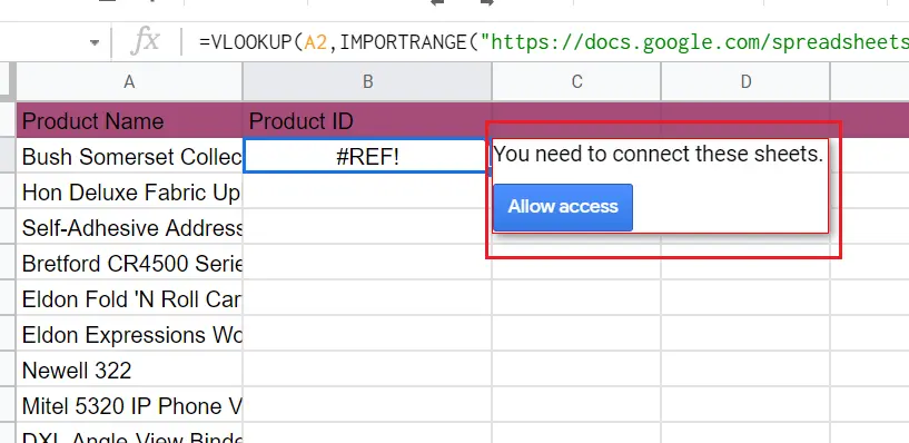
=VLOOKUP(A2,IMPORTRANGE("https://docs.google.com/spreadsheets/d/1Q1q5h6dS2CB7w34NQVd5EkBmHCy4LtwtG3UIvNpLLrU/edit#gid=114008253","Product Name!$A$2:$C$15"),2,)

A2→ Is the cell where my product list starts, corresponding to the product code on the page I am on. I was not using a cell in my table in other headings. I was choosing A2 in the other table. I'm choosing from the table I'm in here

IMPORTRANGE→  I am using this function because I will get data from another workbook. You can find detailed information about the use of this function in the article →"How to use IMPORTRANGE function in Google Sheets?"

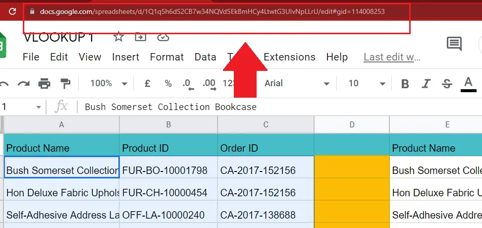
“https://docs.google.com/spreadsheets/d/1Q1q5h6dS2CB7w34NQVd5EkBmHCy4LtwtG3UIvNpLLrU/edit#gid=114008253”→ The URL is of the workbook from which I want to import data

Don't forget to use (") after copy-pasting the URL.

"Product Name!$A$2:$C$15" 🡪 Sheet name and cell range in the other workbook.

1. “page name!
2. The cell range to search. Write by pressing F4. Fix it with $. And end with “ ).

The future column of my data. I'm typing 2 because the product id is in the second column. I want my product id, which is the exact equivalent of the product names, to come. Putting a comma and leaving it blank means the same as False.

After completing the function, we will receive a warning. It asks for permission to access the other workbook. If we do not have access to our workbook, the data does not come. We need to make sure we have access.