How to Use the UNIQUE Function in Google Sheets?

When working with Google Sheets, we may have written the same data in our worksheet more than once. If there are few rows and columns, we can handle this one by one.
But this becomes very difficult when working with very large tables. Suppose there are multiple duplicate data in a worksheet shared with us. By highlighting the repetitions, we can detect these repetitions.
You can find the detailed article about it here: “How to highlight in Google Sheets?” If we want to remove duplicates in our worksheet and work with a clean sheet, we should use the UNIQUE function.
What is the syntax of the UNIQUE function?
The UNIQUE function removes duplicates and brings us clean data in a new column.
There are some points that we should pay attention to here. Because the function gives us a new column, if there are places where we need to get the sum, or if we have two separate columns like first and last name, we may make a mistake. It accepts one because there are two names, but the surnames are different.
After mentioning the places, we need to pay attention to, let's move on to the example.
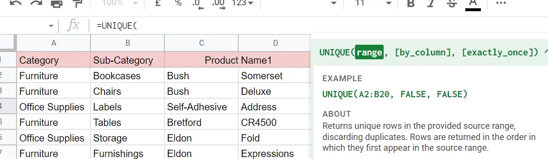
=UNIQUE(cell range)
Typing this brings us the non-repeating rows in column A.
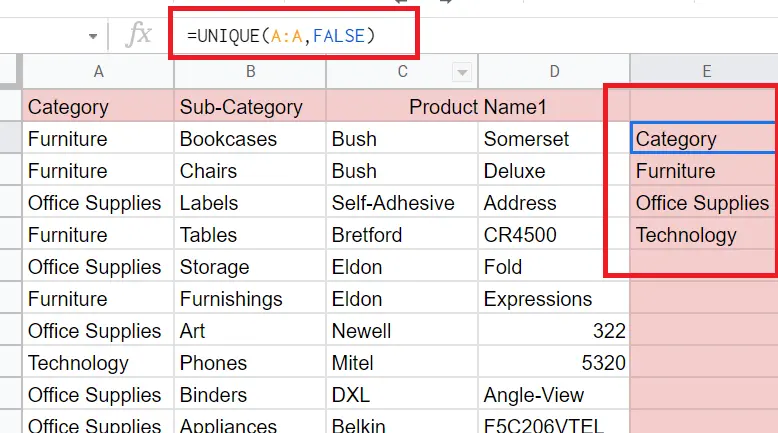
=UNIQUE(cell range, FALSE)
It means the same as above[=UNIQUE(cell range)] Because when left blank, it is assumed to be False.
=UNIQUE(cell range, FALSE, TRUE) →Returns rows that are never repeated in the column. The implementation of the function is as follows.
To use the unique function,
- Go to the column where the results will be sorted
- =UNIQUE(cell range)→ If you want only the non-repeating ones in the column you want
- =UNIQUE(cell range, False, True) →If you want the non-repeatable ones in your column to come
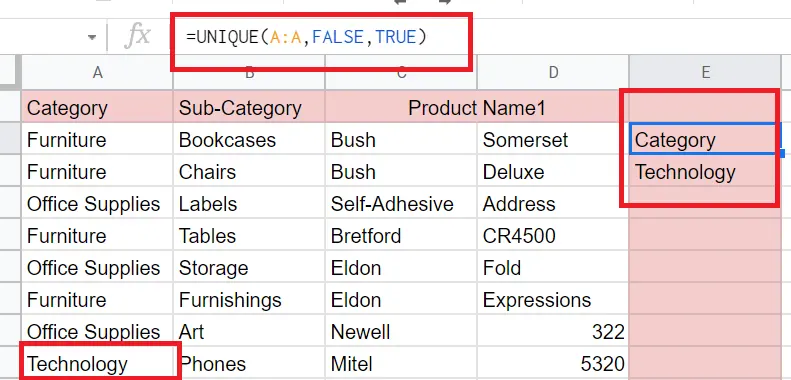
Technology in column A is never repeated. When I specified this in the function, only the technology came.
I want the non-repeating products in the Product Name column to come. Here the column is fragmented, only the header is common. If we trade by looking at column C, we will be doing the wrong trade. Because the rest of the product names are in column D. We need to choose the cell range carefully in the function.
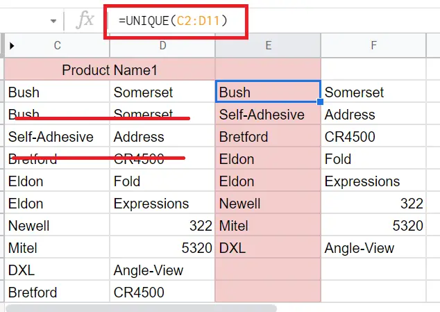
At first glance, ‘Eldon’ seems to have passed twice, but when we look at the other column, the product name continues differently.
If we want to make changes in the new column listed, we will see a warning. If we want to make changes to this new column, then
Right click -> Copy -> Paste Special->Values only
If we don't want the uniques to come in a new column, we can highlight the existing column. You can refer to this article for →"How to highlight in Google Sheets?"
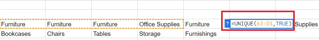
We can apply the UNIQUE function on columns as well as rows. The syntax is as follows.
=UNIQUE(cell ranges, TRUE)