How to filter in Google Sheets?

Working with Google Spreadsheets, we encounter many situations requiring us to search, and our data can be very large. Do not waste your time looking for something at the large table. Filters take care of this for us.  Let's start with the menu first.

How to filter using the menu?

To filter using the menu:

1. Select the cell range you want to filter
2. Menu->Data-> Create a filter

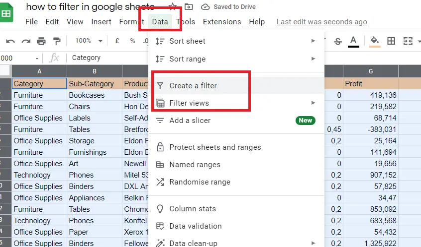
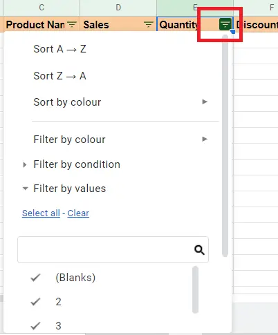
Now the selected cell range is filtered. We can see this with the symbol appearing at the beginning of the line. Let's analyze the screen that appears when we click on the icon.

Detailed text with sorting options in the menu 🡪 “How to sort in google sheets”

With Filter by colour, we can colour the cells we filtered.

We will show an example on 'filter by condition', but please find the detailed article here-> “How to highlight in google sheets?”

With conditional filtering, we can give a certain date range or a certain amount range.

Let's delve into the details with an example. Let's say only rows greater than 4 will come in the amount column.

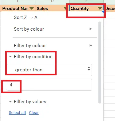
After selecting the cell range and adding the condition, take a look at the new quantity column.

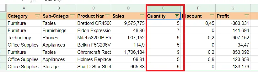
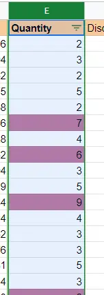
Since only values ​​greater than 4 are displayed in the column, the number of rows has decreased considerably. If we want the column to keep its old state (no unconditional values ​​are removed), we can use the conditional filter. We can see the values ​​we want by assigning them a different colour.

Menu->Data->conditional formatting

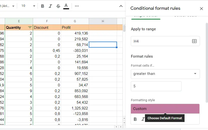
When we select the cell range and type 'only values ​​greater than 5', our column will become:

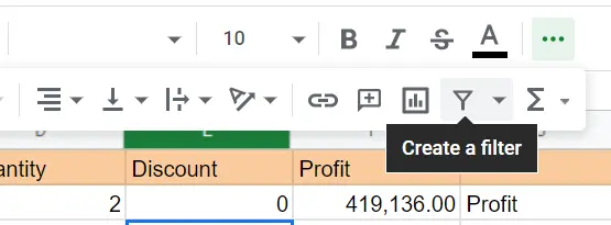
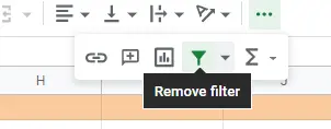
How to filter using the toolbar?

We can attain the filtering by using the toolbar, just as we did by using the menu before.

Toolbar-> Filter icon->Create a filter

When we do it with the menu, the same procedures apply here as well. When clicked on the icon on the side of the column, the same window will appear.

How to filter with filter function?

We can use the menu and toolbar, as well as a filter with '=FILTER()' Here the filtering is done in a new column, not in the current column.

1. Come to the cell in the column from which you want the filtering result to come.
2. =FILTER(cell range, condition1) -> condition can be increased if desired.

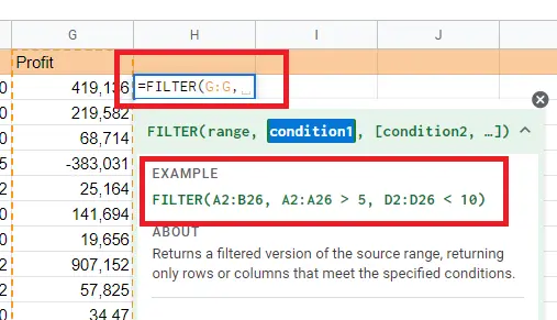
Let's filter the Profit column with the condition 'Profit>600000' I came to column H, which is an empty column because Profit is in my G column.

=FILTER(G:G; G:G>600000)

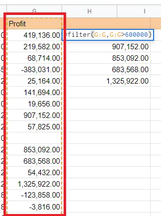
Only profit>600000 came out. The reason why I wrote G: G; is because I chose the entire column, not a specific range. If I select a specific range of cells, it does not include the newly added value in my filter. But in this way, every added value passes to column H if it meets the condition.

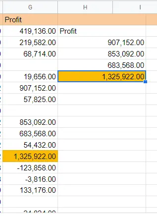
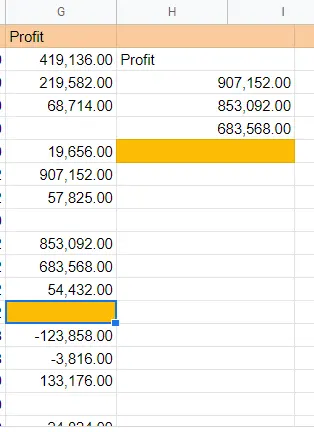
If there is a deletion in column G, providing it is among the values ​​satisfying the condition; it is deleted from column H. It is not possible to delete in column H.

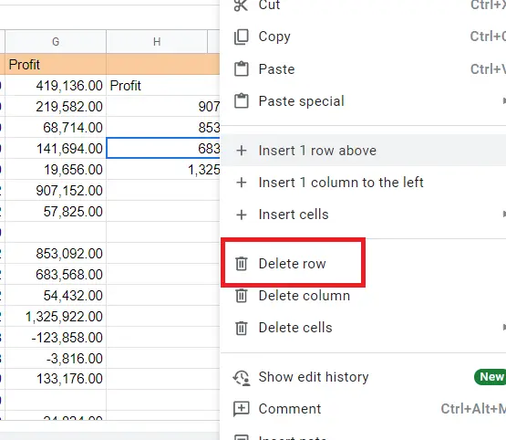
The deleted row will be visible but won't let us delete it. Since the data comes from column G, it only allows deleting cells in column G.

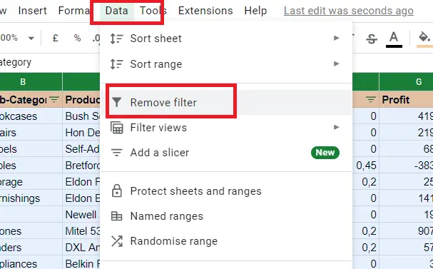
How to remove the filter?

The filter created from the menu or toolbar can be removed from the menu or toolbar with the 'remove filter'.

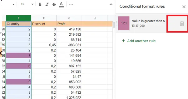
Conditional formatting; this way it is not removed. For this, we need to open the same window and click on the trash can.

Menu->Format-> conditional formatting

Filtering is done with the formula, so it is enough to delete the formula.