How to hide rows in Google Sheets?

There are sometimes too many rows, which you do not need when working with Google Sheets. Therefore you can hide them to avoid confusion.

You can hide a row with a right-click, or with the help of the 'help menu'. Let's take a look at the right click first.

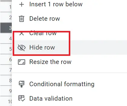
Hiding Rows with Right Click

1. Select the rows you want to hide.
2. Right-click
3. Hide row

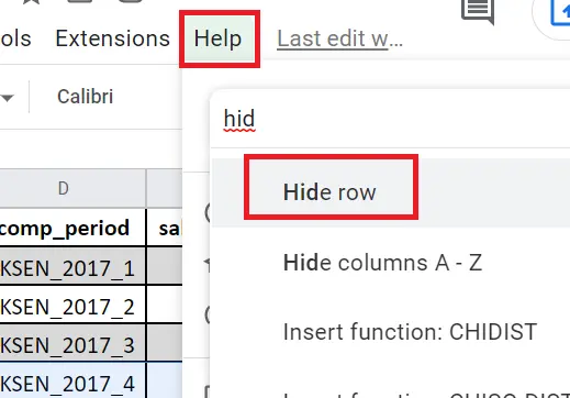
Hiding Rows Using with Help Menu

1. Select the rows you want to hide
2. Click the help menu
3. Write ‘Hide’
4. Click -> Hide Rows

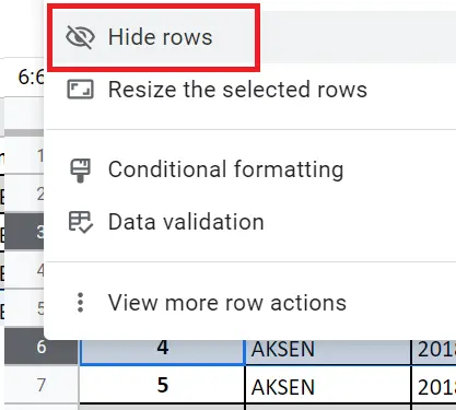
How to Hide Multiple Rows?

The steps for hiding mentioned above are just for a single row. To hide multiple rows, please follow these steps:

1. Hide adjacent rows
2. Go to the rows you want to select
3. While holding down Shift, you can keep selecting to the right or left with the arrow sign; or you can select with the mouse while holding down Shift. For example, we want to select rows A and rows D and in between. If we select rows A first and then rows D while holding down SHIFT, the in-between ones will be automatically selected.
4. Hide a discrete row by selecting the rows you want. Select the other rows while holding down CTRL. In this way, the remaining rows are not selected.

Hiding Rows with a Shortcut

1. Select the rows you want to hide. (Selecting multiple rows mentioned above)
2. Ctrl+Alt+9 (hold down Ctrl + Alt at the same time and press 9).

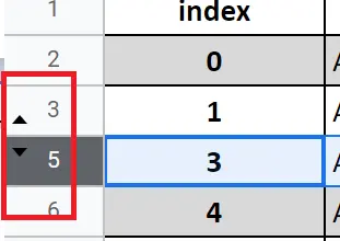
How to Unhide Rows?

How to make hidden rows visible? An arrow appears between the hidden rows. This is the hidden rows indicator. Click on the arrow signs so that signs and rows will become visible again.

That's it for hiding rows. You can find a detailed article about making rows visible here->" How to unhide rows in Google Sheets?"