How to make a table in Google Sheets?

Because Google Sheets acts as a table we do not need to do anything extra to create a table. Therefore, we will only format it.

How to Format Text?

Formatting the headings make them clear in the table. You can choose a different text type for the title, show it bolder.

Aligning a text

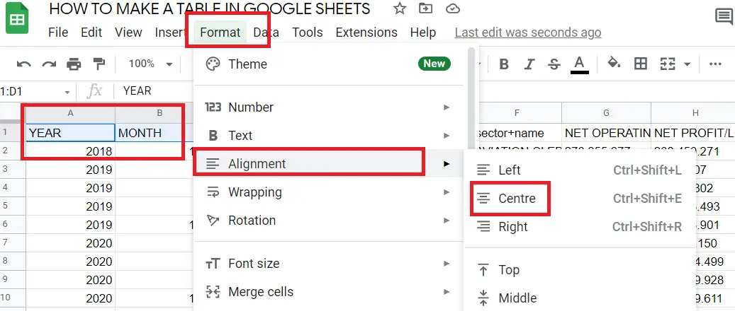
Texts are aligned to the left of the columns. If you want to keep the headers in the middle execute the following steps:

1. Select related cells(headings)
2. Menu->Format->Alignment->Centre

Also, it can be done using the toolbar:

1. Select related cells(headings)
2. Click ‘Horizontal align icon’ in the toolbar-> Centre

Changing the text type

1. Select related cells
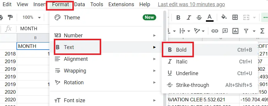
2. Format → Text → I choose bold

How to Format Numbers?

Texts are aligned to the left and numbers are aligned to the right. If a column is placed to the right, we know that it is a number. Some numbers require post-edit. If it is a monetary expression, for instance, the currency can be put next to the number; or we want to indicate it as a decimal, or we can decrement '0'.

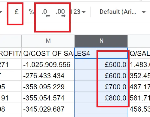
Now let's add currency and reduce zero:

1. Select related cells
2. Toolbar → format as currency
3. Toolbar → increase decimal places

How to Format the Borders?

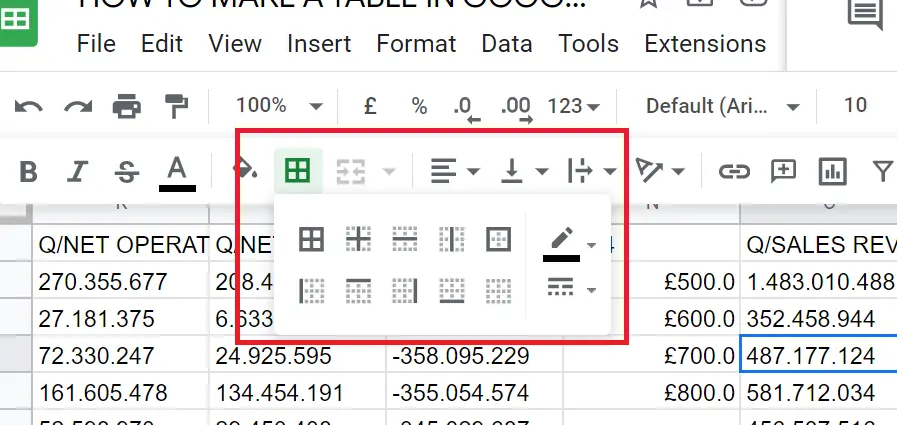
Borders can be added to the tables from the border options:

1. Select related cells
2. Toolbar → Border

How to Do Colouring?

By colouring, we can make titles more outstanding or columns more distinguishable. If the sample, has an index column, we can use a different colour from the table colour to distinguish it. Adjust the text colour according to the cell colours so that it will be easy to read.

How to Colour the Title?

Colouring the titles makes it easier to read. besides, for example; When sorting, we may inadvertently include titles in the order. If it's coloured, we're less likely to make mistakes.

1. Select the column to be sorted (except for the title)
2. Right-click → Sort

To colour the title:

1. Select title
2. Toolbar → Fill colour

How to Colour the Columns?

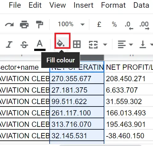
1. Select related column
2. Toolbar → Fill colour
   

How to Make Conditional Colouring?

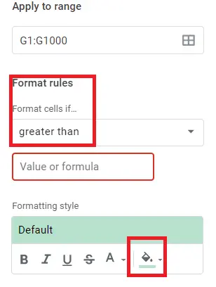
Conditions can be added to the table to make it easier to read. For example, we can set the values ​​below a certain value as x colour and above it as y colour.

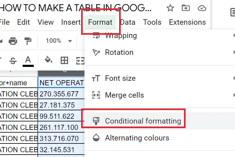
1. Select related cells
2. Menu → Format → Conditional formatting
   

Enter the rule from the pop-up window.

How to Remove Formatting?

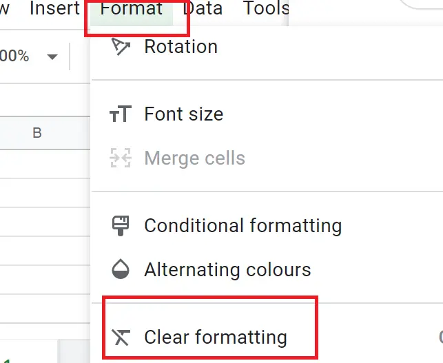
To remove the formatting, respectively; Menu → format → clear formatting