How to indent text in Google Sheets?

In Google Sheets, the text is italicized to the left, and numbers are italicized to the right. When we work with texts, we may want a list view rather than the normal view. Categorizing and indenting texts provides ease of reading. However, there is no shortcut for this function in Google Sheets. But we can do it manually ourselves. I will show you two methods to do this.

Indent by removing border lines

We can indent using the first two columns in our table.

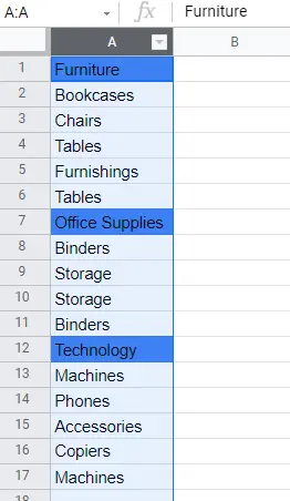
1. Move the data in column A to column B or right-click add a column
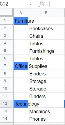
2. Cut the ones you want to be headings (the blue ones) and paste them into column A. (right-click-> cut->paste)

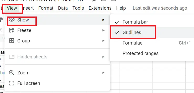
3. Remove borders from the menu. Menu->View->Show->Gridlines

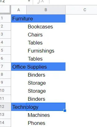
And that's all! There is now text indentation. The old cells are no longer blue because I cut and pasted them here. My titles are blue. To ensure the continuation of the text in the same format, it looks better to format the cells where the text continues in the same way.

How to indent text using the menu?

There is no direct option in the menu. Therefore, we have to add it to the menu ourselves. With this addition, we will be able to indent with one click. Let's see how it is done.

Menu->Format->Number->Custom number format

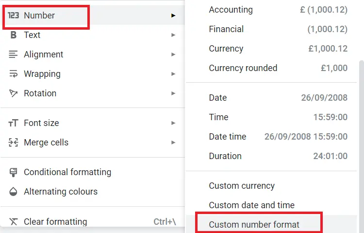
Let's look at the screen that comes up when we click 'Custom number format'

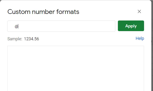
We leave as many spaces as we want to indent for the sub-category in the blank area and put '@'.

I put ' @'  for the example

Now let's go back to our table and select the range of cells we want to indent:

1. Select range of cells
2. Menu->Format-> our special format is saved. We can now indent for each range of cells we select.

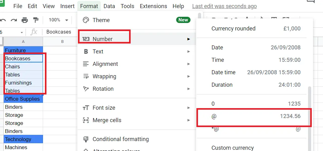
There was no such shortcut in the menu before, but now there is. You can apply it to the cells you want. If you lose this shortcut in the menu;

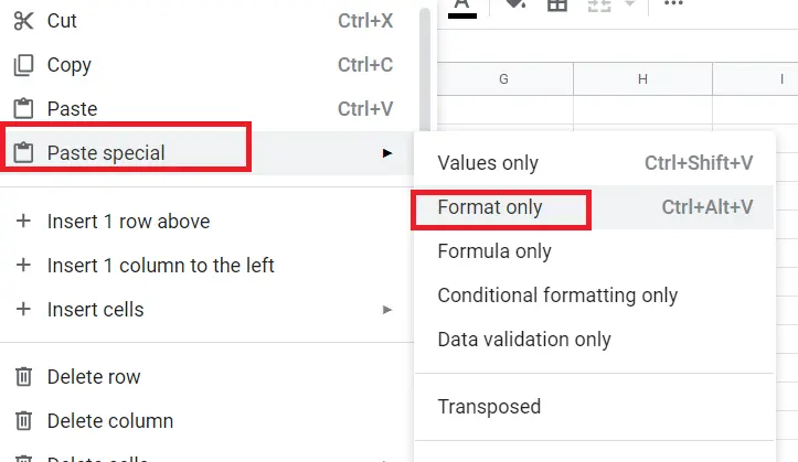
1. Copy the data we indented.
2. Right-click and just copy format. The format of the cells you did this will now change.

These were the methods we used to indent text. I hope it was useful.